Dave Mattingly 4:15 pm on January 27, 2016

Spatial Data, Part 5: Resources

This is part five in a series:

The things we’ve looked at over the last few lessons come from things that I’ve picked up from the people and places that I mention here.

Resources

1. Smart People

Much of what I’ve learned, I learned from these folks:

2. Recursion and Fractals

Simon Greener shows how to make a circle that’s made of circles, with text showing their position. The whole Spatial DB Advisor is filled with amazing tricks.

Alastair Aitchison shows have to draw recursive triangles.

Slava Murygin shows how to make recursive snowflakes.

3. Artwork

Alex Whittles shows how to convert a vector image into geospatial data.

Click these images to see how to make Grinch, a Christmas tree with proper coloring, one with random ornaments, Venus, or a hotel floorplan.

4. Utilities

SQL Magazine offers a quite of utilities to handle a variety of graphic and charting situations.

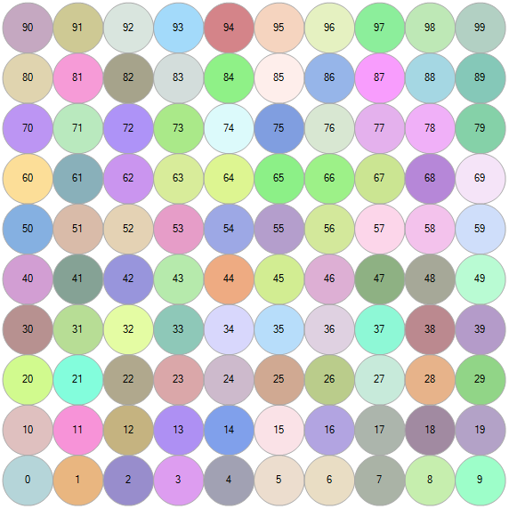
Download here.

5. Color Palette

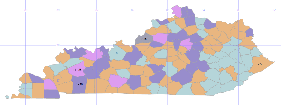
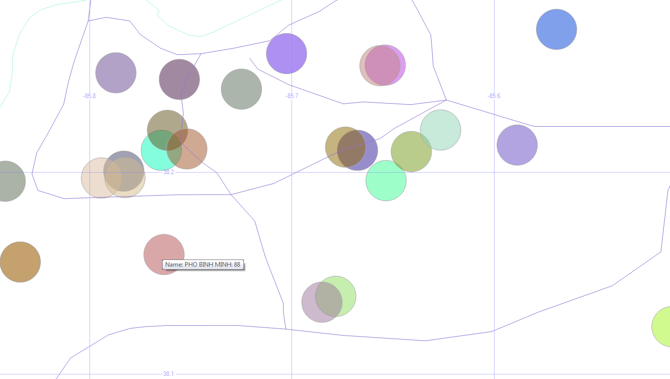
The default color scheme that SQL uses doesn’t always fit the bill. But by specifying the order of the items you display, you can control which one gets which color.

;with n(x) as (select 0 union all select x+1 from n where x < 99)
select cast(x as varchar) label,
geometry::Point(x%10,x/10,0).STBuffer(.5)
from n order by x

The palette ends up looking like this.

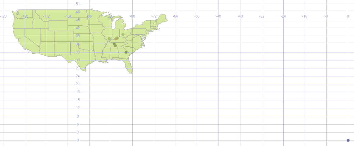
6. Finding Geospatial Data

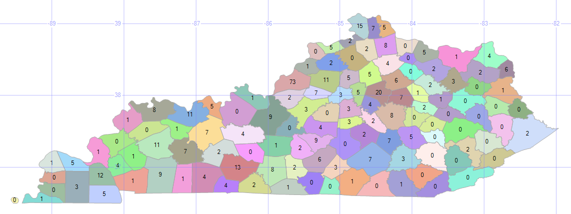
There are many collections of geospatial data available for free (and many more for pay). Being a cheapskate myself, I tend to stick with free as much as possible.

Search for terms like shapefile, geospatial, data, and the region (Kentucky, etc.) and the type of data (geography, roads, elevation, demographics, roads, etc.) that you’re interested in.

I generally prefer to work with .SHP shapefiles, but there are a number of filetypes out there. KML (Keyhole Markup Language) is another popular one.

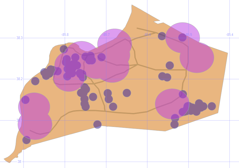
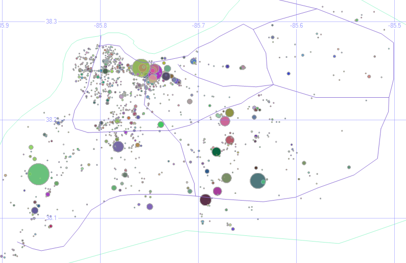
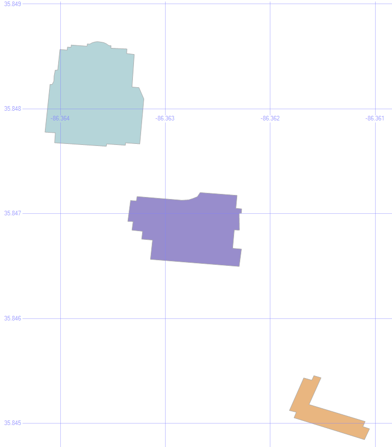
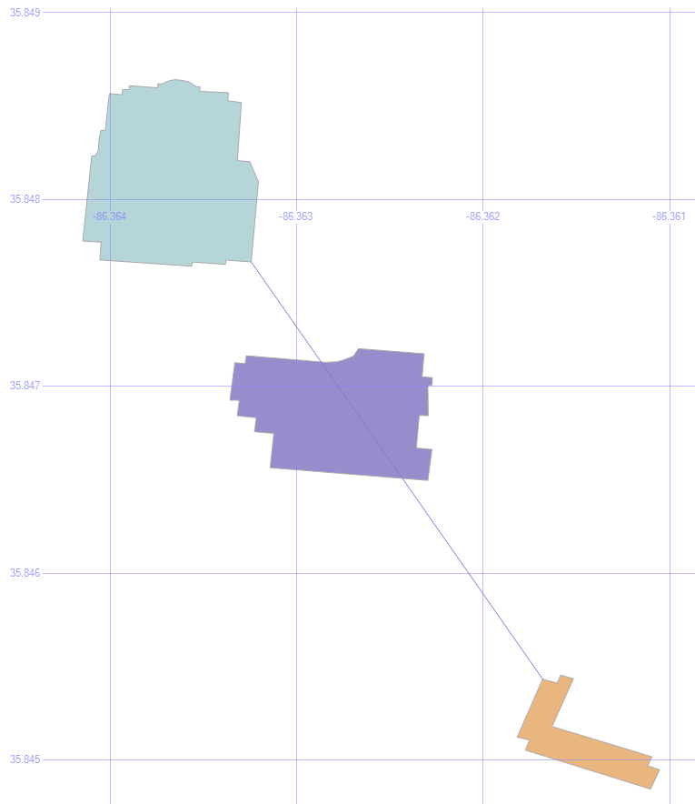
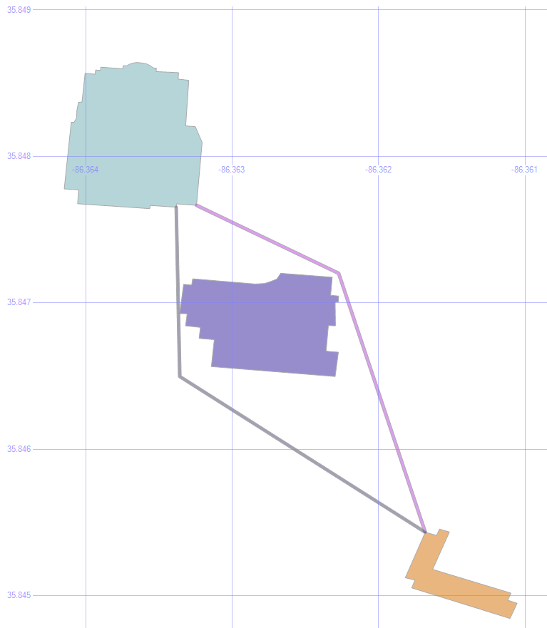
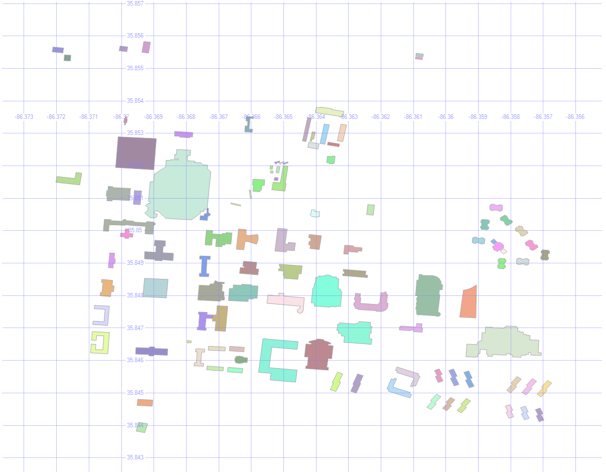
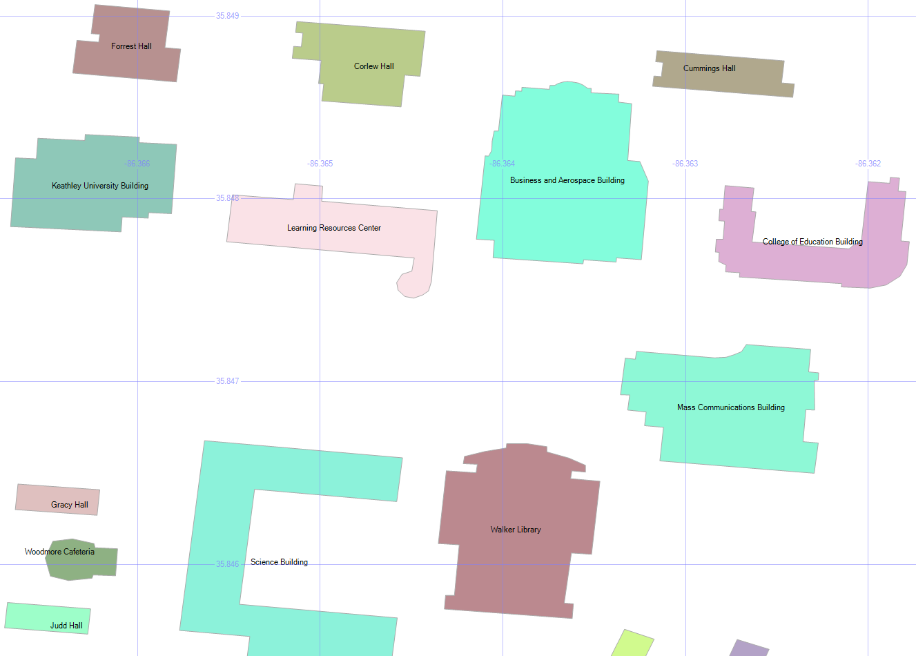
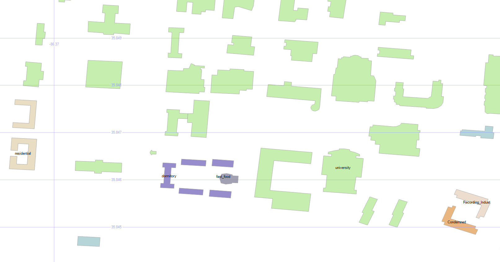
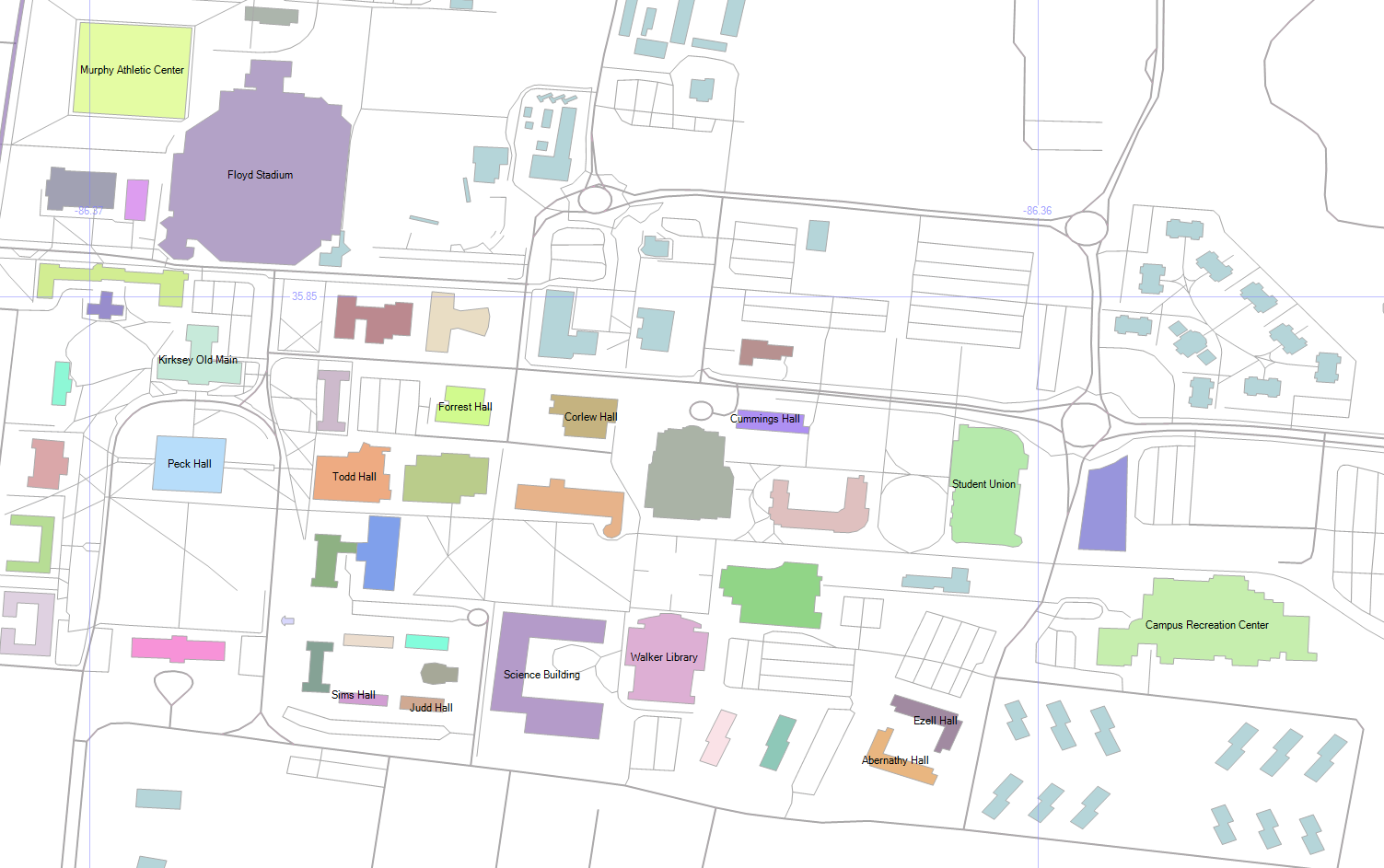
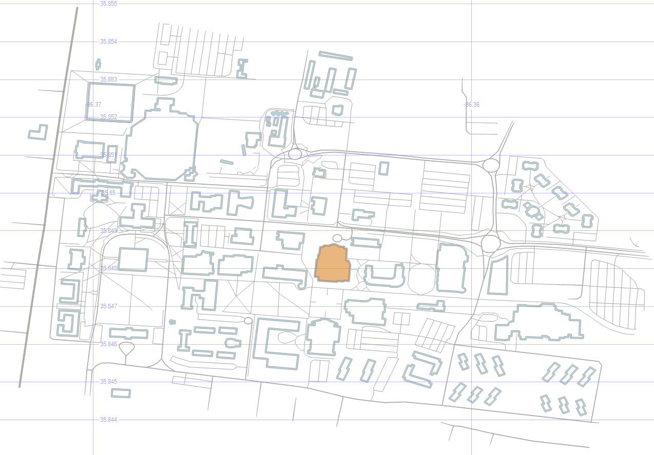
When I get specific local data including buildings (like I did for MTSU in Part 2), I prefer to use the service at bbbike.org, but MapSys gives an overview of the various ways to find and import geospatial data.

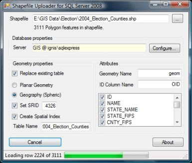
7. Loading Geospatial Data

The tool I prefer for load the data is Shape2SQL from SharpGIS. It’s lightweight and easy to use, and the instructions should handle whatever troubles you might run into.

The one thing to keep in mind is that if you’re loading geographical data, you’ll need to switch the datatype and pick and SRID (usually the default of 4326).

8. A Parting Gift

For a little fun, run this select:

select convert(geometry,'multipolygon (((0.0193705 0.678262, 0.0871671 0.678262, 0.164649 0.290852, 0.251816 0.629835, 0.329298 0.629835, 0.416465 0.281167, 0.493947 0.678262, 0.552058 0.678262, 0.455206 0.194, 0.377724 0.194, 0.290557 0.562039, 0.184019 0.194, 0.106538 0.194, 0.0193705 0.678262), (0.59037 0.678262, 0.658167 0.678262, 0.735649 0.290852, 0.822816 0.629835, 0.900298 0.629835, 0.987465 0.281167, 1.06495 0.678262, 1.12306 0.678262, 1.02621 0.194, 0.948724 0.194, 0.861557 0.562039, 0.755019 0.194, 0.677538 0.194, 0.59037 0.678262), (1.16137 0.678262, 1.22917 0.678262, 1.30665 0.290852, 1.39382 0.629835, 1.4713 0.629835, 1.55847 0.281167, 1.63595 0.678262, 1.69406 0.678262, 1.59721 0.194, 1.51972 0.194, 1.43256 0.562039, 1.32602 0.194, 1.24854 0.194, 1.16137 0.678262), (1.93576 0.329593, 2.06167 0.329593, 2.06167 0.203685, 1.93576 0.203685, 1.93576 0.329593), (2.70046 0.901022, 2.77795 0.901022, 2.77795 0.194, 2.70046 0.194, 2.70046 0.290852, 2.64235 0.223056, 2.59393 0.194, 2.56487 0.184315, 2.50676 0.184315, 2.46802 0.194, 2.42928 0.223056, 2.39054 0.271482, 2.36148 0.368334, 2.36148 0.465186, 2.38085 0.552354, 2.40991 0.610465, 2.45833 0.658891, 2.49707 0.678262, 2.52613 0.687947, 2.59393 0.687947, 2.64235 0.668576, 2.70046 0.62015, 2.70046 0.901022), (2.70046 0.562039, 2.70046 0.348964, 2.62298 0.271482, 2.58424 0.252111, 2.52613 0.252111, 2.48739 0.281167, 2.46802 0.310223, 2.44865 0.368334, 2.44865 0.484557, 2.46802 0.542668, 2.48739 0.581409, 2.51645 0.610465, 2.5455 0.629835, 2.60361 0.629835, 2.65204 0.60078, 2.70046 0.562039), (2.95185 0.658891, 3.01965 0.678262, 3.06807 0.687947, 3.17461 0.687947, 3.21335 0.678262, 3.25209 0.658891, 3.27146 0.629835, 3.29083 0.571724, 3.29083 0.271482, 3.30052 0.252111, 3.31989 0.242426, 3.35863 0.242426, 3.36832 0.203685, 3.32958 0.184315, 3.29083 0.184315, 3.25209 0.203685, 3.22304 0.252111, 3.1843 0.223056, 3.12619 0.194, 3.08745 0.184315, 3.02933 0.184315, 2.99059 0.194, 2.96154 0.21337, 2.93248 0.242426, 2.91311 0.290852, 2.91311 0.348964, 2.93248 0.39739, 2.98091 0.445816, 3.01965 0.465186, 3.08745 0.484557, 3.21335 0.484557, 3.21335 0.562039, 3.19398 0.60078, 3.14556 0.629835, 3.06807 0.629835, 3.00996 0.610465, 2.95185 0.581409, 2.95185 0.658891), (3.21335 0.436131, 3.12619 0.436131, 3.06807 0.41676, 3.02933 0.39739, 3.00028 0.348964, 3.00028 0.300538, 3.01965 0.271482, 3.05839 0.242426, 3.10682 0.242426, 3.16493 0.261797, 3.21335 0.300538, 3.21335 0.436131), (3.46474 0.678262, 3.55191 0.678262, 3.71656 0.281167, 3.88121 0.678262, 3.95869 0.678262, 3.74561 0.194, 3.66813 0.194, 3.46474 0.678262), (4.49579 0.41676, 4.15681 0.41676, 4.15681 0.368334, 4.17618 0.329593, 4.19555 0.300538, 4.24397 0.261797, 4.30208 0.242426, 4.37957 0.242426, 4.42799 0.252111, 4.49579 0.271482, 4.49579 0.21337, 4.42799 0.194, 4.36988 0.184315, 4.28271 0.184315, 4.23429 0.194, 4.16649 0.223056, 4.11806 0.261797, 4.08901 0.310223, 4.06964 0.378019, 4.06964 0.474872, 4.07932 0.523298, 4.09869 0.571724, 4.14712 0.629835, 4.19555 0.668576, 4.26334 0.687947, 4.34083 0.687947, 4.39894 0.668576, 4.43768 0.639521, 4.46673 0.60078, 4.4861 0.552354, 4.49579 0.494242, 4.49579 0.41676), (4.40862 0.474872, 4.15681 0.474872, 4.16649 0.523298, 4.18586 0.562039, 4.2246 0.610465, 4.26334 0.629835, 4.32145 0.629835, 4.3602 0.610465, 4.38925 0.581409, 4.40862 0.532983, 4.40862 0.474872), (4.62127 0.678262, 4.68906 0.678262, 4.68906 0.581409, 4.72781 0.639521, 4.76655 0.678262, 4.78592 0.687947, 4.83434 0.687947, 4.8634 0.658891, 4.88277 0.62015, 4.89245 0.581409, 4.92151 0.629835, 4.95057 0.668576, 4.98931 0.687947, 5.02805 0.687947, 5.0571 0.668576, 5.07647 0.639521, 5.08616 0.591094, 5.08616 0.194, 5.01836 0.194, 5.01836 0.591094, 4.98931 0.62015, 4.96994 0.62015, 4.9312 0.581409, 4.89245 0.513613, 4.89245 0.194, 4.82466 0.194, 4.82466 0.591094, 4.7956 0.62015, 4.77623 0.62015, 4.71812 0.562039, 4.68906 0.513613, 4.68906 0.194, 4.62127 0.194, 4.62127 0.678262), (5.23585 0.658891, 5.30365 0.678262, 5.35207 0.687947, 5.45861 0.687947, 5.49735 0.678262, 5.53609 0.658891, 5.55546 0.629835, 5.57483 0.571724, 5.57483 0.271482, 5.58452 0.252111, 5.60389 0.242426, 5.64263 0.242426, 5.65232 0.203685, 5.61358 0.184315, 5.57483 0.184315, 5.53609 0.203685, 5.50704 0.252111, 5.4683 0.223056, 5.41019 0.194, 5.37145 0.184315, 5.31333 0.184315, 5.27459 0.194, 5.24554 0.21337, 5.21648 0.242426, 5.19711 0.290852, 5.19711 0.348964, 5.21648 0.39739, 5.26491 0.445816, 5.30365 0.465186, 5.37145 0.484557, 5.49735 0.484557, 5.49735 0.562039, 5.47798 0.60078, 5.42956 0.629835, 5.35207 0.629835, 5.29396 0.610465, 5.23585 0.581409, 5.23585 0.658891), (5.49735 0.436131, 5.41019 0.436131, 5.35207 0.41676, 5.31333 0.39739, 5.28428 0.348964, 5.28428 0.300538, 5.30365 0.271482, 5.34239 0.242426, 5.39082 0.242426, 5.44893 0.261797, 5.49735 0.300538, 5.49735 0.436131), (5.9037 0.765429, 5.98119 0.765429, 5.98119 0.668576, 6.20395 0.668576, 6.20395 0.610465, 5.98119 0.610465, 5.98119 0.300538, 6.01024 0.261797, 6.06835 0.242426, 6.16521 0.242426, 6.21363 0.252111, 6.21363 0.194, 6.14583 0.184315, 6.02961 0.184315, 5.96182 0.203685, 5.93276 0.232741, 5.91339 0.261797, 5.9037 0.310223, 5.9037 0.610465, 5.7778 0.610465, 5.7778 0.668576, 5.9037 0.668576, 5.9037 0.765429), (6.4747 0.765429, 6.55219 0.765429, 6.55219 0.668576, 6.77495 0.668576, 6.77495 0.610465, 6.55219 0.610465, 6.55219 0.300538, 6.58124 0.261797, 6.63935 0.242426, 6.73621 0.242426, 6.78463 0.252111, 6.78463 0.194, 6.71683 0.184315, 6.60061 0.184315, 6.53282 0.203685, 6.50376 0.232741, 6.48439 0.261797, 6.4747 0.310223, 6.4747 0.610465, 6.3488 0.610465, 6.3488 0.668576, 6.4747 0.668576, 6.4747 0.765429), (7.16677 0.901022, 7.27331 0.901022, 7.27331 0.794484, 7.16677 0.794484, 7.16677 0.901022), (7.00212 0.678262, 7.26362 0.678262, 7.26362 0.194, 7.18614 0.194, 7.18614 0.62015, 7.00212 0.62015, 7.00212 0.678262), (7.51501 0.678262, 7.59249 0.678262, 7.59249 0.581409, 7.63123 0.629835, 7.67966 0.668576, 7.73777 0.687947, 7.79588 0.687947, 7.83462 0.678262, 7.87336 0.649206, 7.89273 0.610465, 7.90242 0.571724, 7.90242 0.194, 7.82494 0.194, 7.82494 0.552354, 7.80557 0.591094, 7.76683 0.610465, 7.7184 0.610465, 7.66997 0.591094, 7.59249 0.513613, 7.59249 0.194, 7.51501 0.194, 7.51501 0.678262), (8.42499 0.678262, 8.49279 0.678262, 8.49279 0.203685, 8.4831 0.145574, 8.46373 0.0971477, 8.43468 0.0584068, 8.39594 0.0293511, 8.34751 0.00998063, 8.29908 0.0002954, 8.21192 0.0002954, 8.16349 0.00998063, 8.11506 0.0196659, 8.11506 0.0874625, 8.18286 0.068092, 8.23129 0.0584068, 8.30877 0.0584068, 8.3572 0.0777772, 8.38625 0.106833, 8.41531 0.155259, 8.41531 0.300538, 8.37657 0.252111, 8.32814 0.21337, 8.27971 0.194, 8.21192 0.194, 8.16349 0.21337, 8.11506 0.252111, 8.08601 0.300538, 8.06664 0.368334, 8.06664 0.474872, 8.08601 0.552354, 8.12475 0.62015, 8.18286 0.668576, 8.24097 0.687947, 8.30877 0.687947, 8.37657 0.658891, 8.42499 0.62015, 8.42499 0.678262), (8.41531 0.562039, 8.41531 0.358649, 8.37657 0.310223, 8.33783 0.281167, 8.2894 0.261797, 8.25066 0.261797, 8.20223 0.290852, 8.17318 0.329593, 8.15381 0.39739, 8.15381 0.474872, 8.16349 0.523298, 8.19255 0.581409, 8.25066 0.629835, 8.31845 0.629835, 8.36688 0.60078, 8.41531 0.562039), (8.71512 0.901022, 8.98631 0.901022, 8.98631 0.194, 8.90883 0.194, 8.90883 0.84291, 8.71512 0.84291, 8.71512 0.901022), (9.17958 0.678262, 9.26675 0.678262, 9.4314 0.310223, 9.59605 0.678262, 9.66384 0.678262, 9.40234 0.0874625, 9.3636 0.0390363, 9.32486 0.0196659, 9.27644 0.00998063, 9.20864 0.00998063, 9.20864 0.068092, 9.28612 0.068092, 9.32486 0.0971477, 9.38297 0.21337, 9.17958 0.678262), (9.92976 0.329593, 10.0557 0.329593, 10.0557 0.203685, 9.92976 0.203685, 9.92976 0.329593), (10.37 0.678262, 10.4475 0.678262, 10.4475 0.581409, 10.4862 0.629835, 10.5347 0.668576, 10.5928 0.687947, 10.6509 0.687947, 10.6896 0.678262, 10.7284 0.649206, 10.7477 0.610465, 10.7574 0.571724, 10.7574 0.194, 10.6799 0.194, 10.6799 0.552354, 10.6606 0.591094, 10.6218 0.610465, 10.5734 0.610465, 10.525 0.591094, 10.4475 0.513613, 10.4475 0.194, 10.37 0.194, 10.37 0.678262), (11.3478 0.41676, 11.0088 0.41676, 11.0088 0.368334, 11.0282 0.329593, 11.0475 0.300538, 11.096 0.261797, 11.1541 0.242426, 11.2316 0.242426, 11.28 0.252111, 11.3478 0.271482, 11.3478 0.21337, 11.28 0.194, 11.2219 0.184315, 11.1347 0.184315, 11.0863 0.194, 11.0185 0.223056, 10.9701 0.261797, 10.941 0.310223, 10.9216 0.378019, 10.9216 0.474872, 10.9313 0.523298, 10.9507 0.571724, 10.9991 0.629835, 11.0475 0.668576, 11.1153 0.687947, 11.1928 0.687947, 11.2509 0.668576, 11.2897 0.639521, 11.3187 0.60078, 11.3381 0.552354, 11.3478 0.494242, 11.3478 0.41676), (11.2606 0.474872, 11.0088 0.474872, 11.0185 0.523298, 11.0379 0.562039, 11.076599999999999 0.610465, 11.1153 0.629835, 11.1735 0.629835, 11.2122 0.610465, 11.2413 0.581409, 11.2606 0.532983, 11.2606 0.474872), (11.6137 0.765429, 11.6912 0.765429, 11.6912 0.668576, 11.9139 0.668576, 11.9139 0.610465, 11.6912 0.610465, 11.6912 0.300538, 11.7202 0.261797, 11.7784 0.242426, 11.8752 0.242426, 11.9236 0.252111, 11.9236 0.194, 11.8558 0.184315, 11.7396 0.184315, 11.6718 0.203685, 11.6428 0.232741, 11.6234 0.261797, 11.6137 0.310223, 11.6137 0.610465, 11.4878 0.610465, 11.4878 0.668576, 11.6137 0.668576, 11.6137 0.765429)))',0)

Dave Mattingly 7:34 am on January 27, 2016

Parody Music

Back when I was a DJ at WLCV radio, I broadcast the Dr. Demento show every week for several years.

Here are some of my favorite parody bands, specifically only counting artists who base their music on other people’s music and lyrics, not just general comedy musicians (who will come later) or cover bands (also later).

These are “my” bands. The bands that helped shape who I am, roughly in order of how much they mean to me.

Dave Mattingly: The Musical, Part 4

Weird Al Yankovic
- Known For: Eat It, and just about every popular parody in the last 40 years
- Memories: Al has become the pop culture that he mocks, yet remains apart from it; above it, even. If the oddballs of the world ever formed our own nation, Weird Al would be our king. “We don’t need no steenking badgers!”
- Favorite Songs: Dare to be Stupid, Everything You Know is Wrong, White & Nerdy, Word Crimes, Spam, Weird Al Theme Song, Grapefruit Diet, Happy Birthday, Pretty Fly for a Rabbi, Since You’ve been Gone, Dog Eat Dog, Spatula City, CNR

ApologetiX
- Known For: Bethlehemian Rhapsody
- Memories: I never liked the Hootie song upon which it was based, but the first time I heard Naomi Gonna be with Ruth, I know this was a band that I’d be listening to for a long time. One time, they hosted a concert about two blocks from my house! I couldn’t believe how close they’d be. The guitarist, Karl, joked that the singer Jay wrote all the lyrics, which worked out great, since he (Karl) wrote all the music. *rimshot*
- Favorite Songs: Bone Digger, Who’s There, Real Sin Savior, Read Ephesians, Naomi Gonna be with Ruth, Jacob’s Name is Israel, I’m Gonna Feed (500 Mouths), Sufferin’ Just Finished, We’re in a Parody Band

Luke Ski
- Known For: Stealing Like a Hobbit
- Memories: Luke is talented and funny, and a driven hard worker. He performs every week and he releases a new song every month. He organized The FuMP, the Funny Music Project. I even wrote a parody song about him, “With Luke Ski” sung to Eminem’s “Without Me.”
- Favorite Songs: 88 Lines about 44 Simpsons, Christopher Walken Sings Spongebob Squarepants, Crazy Jay, House Party at Arkham Asylum, Keanu Barada Nikto

Big Daddy
- Known For: Monster Mash-Up
- Memories: Writing a parody is tough enough; staying true to the original music and tweaking the words. But Big Daddy keeps the words, and puts in the music from a completely different song, which completely blows me away. My favorite is their working stiffs mash-up of the Money for Nothing lyrics set to the Sixteen Tons music. Brilliant!
- Favorite Songs: Money for Nothing, Safety Dance, Whip It, Once in a Lifetime

Allan Sherman
- Known For: Hello Muddah, Hello Faddah
- Memories: Besides being a humor genius, Allan also voiced the Cat the in the Hat cartoon. Whatta guy. He has so many great songs, it’s hard to pick favorites. For me, though, the songs in which he truly shines are the traditional songs and anthems. Since they’d been around for so long, you’d think that all the funny would have been milked out of them, but he finds new laugh-life in the old standards,
- Favorite Songs: Harvey and Sheila, An Average Song, Mexican Hat Dance, Sir Greenbaum’s Madrigal, Sarah Jackman

Bob Rivers Comedy Corp
- Known For: 12 Pains of Christmas
- Memories: The Bob Rivers group is best know for their Christmas album, that has a number of greats on it like I Am Santa Claus sung to Iron Man. But I’m not a huge Christmas fan, so prefer their more secular tunes. Often the ones leaning toward dark humor.
- Favorite Songs: Wrong Foot Amputated, Your Mouth is like Sam Kinison, A Big Ton o’ Moola, All My Songs are Spoken, Hey Kurt Nice Plot

Carla Ulbrich
- Known For: The Guy Who Changes the Light Bulbs
- Memories: There was a time that I wasn’t sure Carla’s health would let her keep going, but she turned it in fuel for comedy, and became known as The Singing Patient. Her album Sick Humor and her book How Can You Not Laugh at a Time Like This are among my favorites. I usually call her “pancake girl” thanks to her Name song.
- Favorite Songs: I Got Tremors, A Name is a Name, The Force is the Force

Tim Cavanagh
- Known For: 99 Dead Baboons
- Memories: When I saw Tim at a DPMA (Data Processing Management Association) meeting in the ’80s, I was the only guy in the audience shouting out requests. The meeting emcee gave out door prizes “worth well over $1,000,” so Tim brought out a bag of prizes worth “well over $7.” He gave out a rubber dog toy (“Do you have a rubber dog?”), and when I caught up with him after the show, there was still a prize in his bag, which he gave to me. An autographed box of prunes.
- Favorite Songs: I Wanna Kiss Her, Pistons, Dead Russian Leaders, Bible Outlet

Da Yoopers
- Known For: Second Week of Deer Camp
- Memories: Da Yoopers have many originals, almost pushing them into the general funny music category instead of this list, but the parodies that they do have are some of my snowy favorites. Rusty Chevrolet has described most of the vehicles I’ve ever owned, Chevy or not.
- Favorite Songs: Rusty Chevrolet, Chiquito War, Fishin’ wit Fred, My Car Won’t Go

Runners Up: Homer and Jethro, Spike Jones, Stan Freberg, Smothers Brothers

Go back to Part 3: Alt Rock or on to Part 5: A Cappella.

Dave Mattingly 6:30 pm on January 26, 2016

Cool Job: NASA

Oh, the humanity!

I’ve done a lot of things for a living over the years, and one of my first was also one of the coolest.

Cool Job, Part 1: NASA

On 1/28/86, the space shuttle Challenger blew up.

Later that year, I got a call from NASA with a job offer, which I accepted. Over the phone. They didn’t realize I had an orange mohawk. I was still a teenager, after all. Ya gotta live.

A few months after that, I moved down to Florida to work at Kennedy Space Center, where I worked in the Mission Planning Office and helped write the software that scheduled shuttle launches, landings, and maintenance.

Capt. Kirk: “No, I’m from Iowa. I only work in outer space.”

I got a haircut before starting, and looked like a real person. But before long, I was back to my old cranial tricks.

My office is visible in all of the footage used in the movies. That one giant building that’s always shown is the VAB – the Vehicle Assembly Building. It’s the mechanic’s garage where the shuttle goes for its oil changes and other maintenance.

My job was actually in NASA’s “Trailer Park.” There were some old railroad cars pushed together sideways with the open sliding doors lined up, making a large single office with branching rooms, sort of. It was a cheap way to use old equipment to make something new-ish. It was air-conditioned, carpeted, and otherwise very nice inside, but I found it amusing that it was practically made of garbage.

When we went back into space the following year, I got to stand on my office rooftop to watch the launch. The vibrations shook my whole body. It was amazing.

I didn’t like Florida, so once we got back into space, I considered my work done, and I moved a thousand miles north so I could do some other nifty tech stuff instead. More on that in my next cool job installment.

The stars look very different today.

But writing space shuttle software for NASA as a teenager is certainly a powerful feather in anyone’s geek cred hat.

Go on to Part 2: Wolf3D

Dave Mattingly 1:04 pm on January 26, 2016

A Reason for Hope

I’m a Christian, and sometimes a teacher/preacher.

Here’s a look at my own story of coming to Christ. This is a very personal story, and won’t necessarily have the wide applicability of some of my other sermons and lessons. I encourage all of you to map out your own walk with Christ.

A Reason for Hope

The Bible tells us to “always be prepared to give an answer to everyone who asks you to give the reason for the hope that you have.” I am ready. In fact, that 1 Peter 3:15 verse is a good summary of my testimony.

“Come, let us reason together,” says the Lord. (Isaiah 1:18)

Rebel

I grew up as a rebel. The world stank, and I didn’t like it. I fought the world by looking and acting different, by arguing and debating, and by spending time on what many would consider the wrong side of the tracks.

In those days Israel had no king; everyone did as they saw fit. (Judges 21:25)

Engineer

I was a math and science whiz, and got my college degree in engineering math and computer science, to better understand the physical and digital worlds. I also minored in psychology and philosophy, to better understand the mind and reality. Over the years, I’ve worked for NASA, Homeland Security, some intelligence agencies that shall go unnamed, virtual reality tech, and many other brainy ‘science-y’ places.

Where were you when I laid the foundations of the earth? Tell me, if you know so much. (Job 38:4)

Atheist

I stopped believing in God as a young’un. I believed that “In the beginning was nothing, which then exploded.” When we die, we turn to dust, and that’s that. My time surrounded by rebels and engineers only served to bolster my own opinion.

Only fools say in their hearts, “There is no God.” They are corrupt, and their actions are evil. (Psalms 53:1)

Scribe

Although I didn’t care much for writing while I was in school, I found after college that I rather enjoyed it. I went on to write hundreds of articles for magazines and newspapers, and after coauthoring some books even founded my own publishing company. Every writer is also a voracious reader, and I was no exception.

See what large letters I use as I write to you with my own hand! (Galatians 6:11)

Oddball

After awkwardly trying to fit in growing up, I realized that I wasn’t meant to be like everyone else, and I sort of liked it that way. I am what I am, and that’s all what I am, as the Sailor Man would say.

They admitted that they were strangers and aliens on earth. (Hebrews 11:13)

Nerd

And of course, I was into all the various nerdy things. Comic books and cartoons, Monty Python, games and toys, science fiction and fantasy, Weird Al, and such. Different from most people, at least at the time. (Nerds are enjoying a bit of a golden age at the moment.)

God gave Joseph unusual wisdom. (Acts 7:10)

Encounter with Christ

That’s who I had been. A weirdo. (Well, I still am a weirdo.)

But my life turned around when I went into business with a Christian who was a real Christian.

Homayoun Sarabi was an engineer from Iran, and was also a Christian. (None of the ‘normal’ American Christians could reach me; God had to import a guy.) We went into business, and were often on the road together. While on the road for business events, often on the weekends, “Homer” would politely invite me to church with him and I’d politely decline.

Over time, the peace and joy that I saw in his life, and the obvious care he had for those around him drew me in. One day in North Carolina, I did go to church with him, and accepted that altar call (the first I’d ever heard).

Holy Spirit

My eyes were opened, and my heart was thirsty for the Lord. I read the scripture. I went to worship. I learned at Bible studies. I took classes at church. My soul was on fire, and I couldn’t get enough.

No one can see the kingdom of God unless they are born again. (John 3:3)

Overhaul

Similar to an addict who knows when he’s hit rock bottom, I couldn’t kid myself that I was “doing okay” and could ease into walking with the Lord. My life’s direction did a full 180, and I turned some heads doing it. Not quite to the extent of Paul in Acts 9:26, but drastic enough for me.

If anyone is in Christ, he is a new creation. The old has gone, the new is here. (2 Corinthians 5:7)

Hey, wait a minute. That’s a porpoise!

Purpose

Now instead of being a collection of chemical reactions drifting inevitably toward oblivion, I felt that there was a reason behind my existence. God had me — specifically me — here for a some particular part of his plan.

Who knows but that you have come to your royal position for such a time as this? (Esther 4:14)

Evangelism

Now, I use my nerdy background to reach out to the freaks, geeks, and weirdo of the world. My people.

Through groups like the Christian Gamers Guild, Fans for Christ, Game Church, and Grave Robbers, plus my own activities in the local community, I can set up church services at comic cons, sci-fi cons, gaming cons, and other gatherings of my fellow oddballs. As “one of their kind” I can speak to them without being some outside churchy guy trying to horn in on their lives. I’m already part of their lives. Because they are me. Weird and loved.

I have become all things to all people so that by all possible means I might save some. (1 Corinthians 9:22)

Summary

I can give a reason for my hope because of who I was, and because of who I am.

R – Rebel
E – Engineer
A – Atheist
S – Scribe
O – Oddball
N – Nerd

H – Holy Spirit
O – Overhaul
P – Purpose
E – Evangelism

Download

Download the PowerPoint.

Learn how I use my testimony to reach others at All Things to All Men.

Dave Mattingly 7:13 am on January 26, 2016

Spatial Data, Part 4: Data Sets

This is part four in a series:

Besides just looking around at geographical features like states, roads, and buildings, we can incorporate human-centric data like restaurants, crimes, and more.

Data Sets

1. Toxic Release Inventory

A “TRI” as reported by the EPA is a Toxic Release Inventory. This could be a chemical spill or some other accident that’s not in our best health interests. Here are the incidents that took place in Kentucky over a ten-year period.

select geometry::CollectionAggregate(geom)
from ky_counties
union all
select geom.STBuffer(.05)
from ky_tri
where geom.STWithin((select geom from us_stateshapes where state = 'KY')) = 1

The EPA offers an interactive map of TRI’s around the country here.

2. Toxic Incidents in Jefferson County

select geometry::CollectionAggregate(geom).STBuffer(.001)
from ky_interstates where geom.STWithin((select geom from ky_counties where id = 24)) = 1
union all 
select geometry::CollectionAggregate(geom) from ky_counties where id = 24
union all
select geom.STBuffer(.01) from ky_tri where geom.STWithin((select geom from ky_counties where id = 24)) = 1

Bringing it close to home, here are the incidents that have taken place in my own hometown of Louisville, KY.

3. Add in the Sirens

select geometry::CollectionAggregate(geom).STBuffer(.001)
from ky_interstates where geom.STWithin((select geom from ky_counties where id = 24)) = 1
union all 
select geom from ky_counties where id = 24
union all
select geometry::UnionAggregate(geom.STBuffer(.01)) from ky_tri where geom.STWithin((select geom from ky_counties where id = 24)) = 1
union all
select geometry::UnionAggregate(geom.STBuffer(.02)) from ky_sirens

The siren radius is an estimate, since the hearing distance can depend on a lot of factors. Still, it’s disturbing to see that there are some parts of the county that have had several incidents but have no sirens for tens of miles. The I-65 corridor on the southern half of Louisville has its share of problems, but no active alert system.

4. Toxic Incidents per County

;with tox (id, ct) as
(select c.id, count(*) from ky_counties c join ky_tri t on c.geom.STContains(t.geom) = 1 group by c.id)
select c.geom, isnull(tox.ct,0) Incidents
from ky_counties c
left outer join tox on c.id = tox.id

By counting the number of incidents per county in a CTE, and joining that to the county map, we can display that number on the SQL map.

On the good side, it’s good to see that there are several counties with zero incidents; on the bad side, 73 in my county? Ouch.

5. Toxic Incident Range Bands

select geometry::CollectionAggregate(geom), '0' Incidents
from ky_counties c where c.id not in (select id from tox) union all
select geometry::CollectionAggregate(geom), '< 5'
from ky_counties c inner join tox on tox.id = c.id where tox.ct < 5 union all
select geometry::CollectionAggregate(geom), '5 - 10'
from ky_counties c inner join tox on tox.id = c.id where tox.ct between 5 and 10 union all
select geometry::CollectionAggregate(geom), '11 - 25'
from ky_counties c inner join tox on tox.id = c.id where tox.ct between 11 and 25 union all
select geometry::CollectionAggregate(geom), '> 25'
from ky_counties c inner join tox on tox.id = c.id where tox.ct > 25

Seeing the individual numbers is informative, but divvying up the data into range bands can make it easier to find patterns and trends.

Since we aggregated the counts into just five range bands, they’re considered just five objects, and therefore only five labels appear.

The southeast part of the state looks pretty good, with mostly light blue zeros and a scattering of tan lows. There’s an almost solid dark blue of tens riding up along I-75. And, if I had to present this kind of bad news to my boss, you can see that I’ve cleverly downplayed Louisville’s 73 TRIs into an “over 25” category.

6. Low Food Scores

;with s (id, dt) as
(select establishmentid, max(inspectiondate) from ky_food
where typedescription = 'food service' group by establishmentid)
select geom.STBuffer(.01) Geom, establishmentname + ': ' + convert(varchar,f.score) Name
from ky_food f 
inner join s on f.establishmentid = s.id and f.inspectiondate = s.dt
where score < 90
union all
select geometry::CollectionAggregate(geom), ''
from ky_interstates where geom.STWithin((select geom from ky_counties where id = 24)) = 1
union all
select geom.STBoundary(), '' from ky_counties where id = 24

Instead of the bad stuff that we may inadvertently breathe and drink due to industrial accidents or chemical spills, let’s look at the bad stuff that we put into our bodies on purpose. Here are the restaurant health inspection codes (usually the “A” papers that we see posted) that are not up to the A level (score < 90).

Here, I’m plotting the low-grade restaurants (using a CTE because I only want the most recent inspection date for each restaurant) around the city, and setting the hover-text to be the name and score.

The data I’m using is from early 2015. So Phi Binh Minh (and the others) might have an “A” in the window these days. Don’t take my map as a food critic review.

7. Violent Crimes in Jefferson County

select geom.STBuffer(.001), left(Crime,1) Crime, convert(varchar,IncidentDate,111) Date
from ky_crime
where geom.STWithin((select geom from ky_counties where id = 24)) = 1
and crime in ('homicide', 'aggravated assault', 'simple assault') and year(incidentdate) = 2014
union all
select geometry::CollectionAggregate(geom), null, null
from ky_interstates where geom.STWithin((select geom from ky_counties where id = 24)) = 1
union all
select geom.STBoundary(), null, null from ky_counties where id = 24

More bad news! Sorry.

Here are the violent crimes in town (thankfully, relatively few homicides) over the course of a year, with the first letter of each of those crimes in our hover-text.

The west end, downtown, and the airport region seem to have the worst of it.

8. Violent Crimes in Jefferson County with Bubble Sizes

;with siz (lat, lon, sz) as
(select latitude, longitude, count(*) size from ky_crime where crime in ('homicide', 'aggravated assault', 'simple assault') group by latitude, longitude)
select geom.STBuffer(sz * .0003) from ky_crime c 
inner join siz on c.latitude = siz.lat and c.longitude = siz.lon
where crime in ('homicide', 'aggravated assault', 'simple assault')
and geom.STWithin((select geom from ky_counties where id = 24)) = 1 and sz > 1
union all
select geometry::CollectionAggregate(geom)
from ky_interstates where geom.STWithin((select geom from ky_counties where id = 24)) = 1
union all
select geom.STBoundary() from ky_counties where id = 24

Instead of just seeing where they are, how about we highlight the dangerous parts of town by making each dot (an address where a crime happened) wider for every crime that happened there, and ignore the dots where only one crime happened. The previous maps showed us which parts of town are dangerous, but this shows us which specific places are “repeat customers” for crimes.

Of course, even one violent crime is too many. And my filename for this image (KY Crime Bubbles) sounds like a street gang made up of clowns or janitors.

The underlying data shows that one of the larger circles could actually be removed. The puke-green circle around the center of the second grid square is some sort of default address for the city. The address is listed simply as “Louisville Metro.” Even so, we learn a lot by plotting our own data on a map like this.

9. Reported Crimes (Bad Geo)

select geom.STBuffer(.5), crime, convert(varchar,IncidentDate,111) Date
from ky_crime
where geom.STWithin((select geom from us_stateshapes where state = 'KY')) = 0
union all
select geometry::CollectionAggregate(geom), null, null from us_stateshapes

So far, I’ve been limited the data displayed just to what happens within Louisville/Jefferson County, but sometimes crimes get reported to the Louisville Metro Police that take place out of town.

Oh, and there are a lot of crimes (32 of them, not all that many compared to the overall volume, really) that happen way out in the middle of the ocean. Actually, no. That’s location 0, 0 (one of those 0’s is the equator, and the other is the prime meridian, which is also where the GMT time zone starts). If no geodata was recorded with the incident, many systems will default it to there. For data like that, you can ignore it or correct it by geocoding it (assigning a latitude and longitude to an address). There are some services that will do that for free, for a given amount of addresses (google maps will geocode 10,000 per day, for example), and other services that will geocode for a fee.

Data Sources

Here are the data sets use for this lesson (the us_stateshapes, ky_counties, and ky_interstates have appeared previously.)

TRI data is here.
Siren, food, and crime data (and dozens of other Louisville data sets) are here.

Getting Involved

I encourage all of you to join in this year’s National Day of Civic Hacking, which is sponsored by the White House’s data.gov open data portal. It’s an annual event put on by the Code for America Brigade to build apps in a single day with other local coders / designers / data’ers, primarily based on using open data sets.

In Louisville, in the past few years, we’ve had apps that:

rate the safety of the neighborhood you’re in
find a particular adoptable animal close to you
aggregate techie calendars from meetup, eventbrite, and more
and dozens more

Your area might also have a chapter of MapTime, which uses and enhances geodata in a variety of ways.

Dave Mattingly 4:47 pm on January 25, 2016

Alt Rock

Here are some of my favorite punk, post-punk, pre-industrial, goth rock, early alternative, dark wave, and such. It’s a little harder for me to put a clean label on what this is, so the somewhat nondescript “alt rock” it is, primarily pulled from the ’80s and ’90s.

These are “my” bands. The bands that helped shape who I am, roughly in order of how much they mean to me.

Dave Mattingly: The Musical, Part 3

Simon F
- Known For: I Want You Back
- Memories: Simon F’s guitarist was Steve Stevens, from Billy Idol’s band. To many, that pegged Simon F as a Billy Idol wannabe or ripoff. To me, he was far more than that. Growing up as an atheist, A Million Miles from Happiness became a personal anthem for a long time. But it’s the defiant pain in Here Comes My Laugh and other songs that keeps me coming back. Sort of a musical equivalent of William Ernest Henley’s “Invictus” poem.
- Favorite Songs: Here Comes My Laugh, A Million Miles from Happiness, American Dream, Love Bomb, New York Girl, Get Out of London, Prisoner of Love

Big Black
- Known For: The Model
- Memories: Steve Albini has been one of the most influential figures in underground indie rock, first as a musician in Big Black, then, Rapeman, then Shellac. But it’s his engineer and producer credits that make him a giant — well over a thousand album, including the Breeders, the Pixies, the Stooges, and so many more. The title of their Songs About F***ing album would lead to many interesting conversations in record stores.
- Favorite Songs: Precious Thing, Colombian Necktie, Bad Penny, The Power of Independent Trucking

Ministry
- Known For: (Every Day is) Halloween
- Memories: Ministry’s cynical outlook and harsh instrumentation was a great channel for my young rage. Especially during my years at NASA’s Kennedy Space Center, Ministry had a prominent place in my playlist rotation (mix tapes, in those days). I still listen to “Over the Shoulder” all the time, especially the 12-inch mix that I have linked below.
- Favorite Songs: Over the Shoulder, The Nature of Love, Angel

Clash
- Known For: Should I Stay or Should I Go?
- Memories: The Clash has had a wide reach. At various times, they were popular on pop charts, classic rock, and on MTV. With such a large catalog of great songs, and with the staggering influence they’ve had, it’s hard to believe they were only together for ten years. Also, the bassist Paul Simonon married Pearl E Gates from Pearl Harbour and the Explosions, which was featured in my new wave list.
- Favorite Songs: Radio Clash, Rock the Casbah, Bankrobber, Rudie Can’t Fail

Ramones
- Known For: Blitzkrieg Bop
- Memories: The Ramones had, if anything, more impact on the musical world than the Clash, although not quite the personal impact on me. Even reaching into pop culture like comic books and the Simpsons.
- Favorite Songs: I Wanna Live, I Wanna be Sedated, Needles and Pins, Spider-Man, Sheena is a Punk Rocker

Runners Up: Foetus, Shriekback, Steriogram, PJ Harvey, Psychic TV, Megadeth

Go back to Part 2: Quirky Music or on to Part 4: Parody Music

Dave Mattingly 1:42 pm on January 23, 2016

Spatial Data, Part 3: Getting Around

This is part three in a series:

Now that we have some local buildings represented in our database, let’s move around.

Getting Around

0. Get the Buildings

In the last step of Part 2, we saved three buildings into temp tables — #orig, #bloc, and #dest.

1. Shortest Path

select geom from #orig union all select geom from #dest union all select geom from #bloc union all
select (select geom from #orig).ShortestLineTo((select geom from #dest))

Let’s Find the Shortest Path to that Condemned Building.

The .ShortestLineTo method will find the shortest path, even taking into account the shapes of the buildings.

But it doesn’t care about any obstacles in its path, which is why we also stored that blocking building to continue our experiment.

2. Put an Envelope on the Obstacle

select (select geom from #bloc).STEnvelope().STBoundary()
union all select geom from #orig union all select geom from #dest union all select geom from #bloc

An envelope will look at the highest and lowest values for the height and the width of an object, and draw a box using those values. We can use this to help find a path around the obstacle.

3. Draw the Corners of the Envelope

select geom from #orig union all select geom from #dest union all select geom from #bloc union all
select geometry::Point((select geom from #bloc).STEnvelope().STPointN((1)).STX, (select geom from #bloc).STEnvelope().STPointN((3)).STY, 0).STBuffer(.0001) union all
select geometry::Point((select geom from #bloc).STEnvelope().STPointN((3)).STX, (select geom from #bloc).STEnvelope().STPointN((3)).STY, 0).STBuffer(.0001) union all
select geometry::Point((select geom from #bloc).STEnvelope().STPointN((3)).STX, (select geom from #bloc).STEnvelope().STPointN((1)).STY, 0).STBuffer(.0001) union all
select geometry::Point((select geom from #bloc).STEnvelope().STPointN((1)).STX, (select geom from #bloc).STEnvelope().STPointN((1)).STY, 0).STBuffer(.0001)

This command illustrates where the corners of that envelope are. After all, we don’t really want the entire envelope to find a way around the obstacle, just the endpoints.

4. Save Those Corners

if object_id('tempdb.dbo.#corn', 'u') is not null drop table #corn create table #corn (geom geometry)
insert into #corn
select geometry::Point(geom.STEnvelope().STPointN((1)).STX, geom.STEnvelope().STPointN((3)).STY, 0) from #bloc
union all
select geometry::Point(geom.STEnvelope().STPointN((3)).STX, geom.STEnvelope().STPointN((3)).STY, 0) from #bloc
union all
select geometry::Point(geom.STEnvelope().STPointN((3)).STX, geom.STEnvelope().STPointN((1)).STY, 0) from #bloc
union all
select geometry::Point(geom.STEnvelope().STPointN((1)).STX, geom.STEnvelope().STPointN((1)).STY, 0) from #bloc

Let’s save those into some temp tables, too, to make the following statements a bit easier to read.

5. Paths to the Corners

select geom from #orig union all select geom from #dest union all select geom from #bloc union all
select o.geom.ShortestLineTo(c.geom).STBuffer(.00001) from #orig o left outer join #corn c on 1=1

Being a method, the .ShortestLineTo can be applied to as many shapes (or points) that we want to give it, all in a single command.

By putting the corners into a temp table, we can draw all four lines at once.

6. Eliminate Overlaps

select geom from #orig union all select geom from #dest union all select geom from #bloc union all
select o.geom.ShortestLineTo(c.geom).STBuffer(.00001)
from #orig o left outer join #corn c on 1=1 left outer join #bloc b on 1=1
where o.geom.ShortestLineTo(c.geom).STIntersects(b.geom)=0

One of those paths goes through the building, which isn’t any help in getting around it. So by added a where clause so that .STIntersects is false, we only see the lines that don’t collide with the building.

Cool! We’re halfway there.

7. Add the Destination

select geom from #orig union all select geom from #dest union all select geom from #bloc union all
select o.geom.ShortestLineTo(c.geom).STUnion(c.geom.ShortestLineTo(d.geom)).STBuffer(.00001)
from #orig o left outer join #corn c on 1=1 left outer join #bloc b on 1=1 left outer join #dest d on 1=1
where o.geom.ShortestLineTo(c.geom).STIntersects(b.geom)=0
and c.geom.ShortestLineTo(d.geom).STIntersects(b.geom)=0

Since those three valid paths are also just geometric data objects, we can use them as the new “origin” for the next leg of our journey.

So, by finding the shortest lines from those lines to the destination building, joining the two line segments into a single object with the .STUnion method, we get:

If we were to apply the .STDistance() method to those paths, we’d see that the purplish path is 4.732 meters, and the blueish path is 5.055 meters.

Shortest Path

Typically, of course, the shortest path problem is focused on roads, not taking shortcuts through the grass.

That’s already been solved in a variety of ways. The most common approach is Dijkstra’s Algorithm.

Here are a couple of SQL implementations: one from Peter Larsson, and one from Hans Olav.

The key to making it quick is generally to pre-calculate all the distances. To a point. Computers these days can’t store the distance from every point on Earth to every other point on Earth, any more than every possible chess move on every board.

Dave Mattingly 8:16 am on January 23, 2016

Quirky Music

Back when I was a DJ at WLCV radio, on the air I was known as “New Wave Dave.”

I developed a taste for oddball music, and here are some of my favorites. Much of this is music that just leaves my friends scratching their heads at how it could even have gotten recorded, much less that it’s anyone’s favorite.

These are “my” bands. The bands that helped shape who I am, roughly in order of how much they mean to me.

Dave Mattingly: The Musical, Part 2

Ed’s Redeeming Qualities
- Known For: Lawn Dart
- Memories: Minimalist, witty, sarcastic, insightful, sad, goofy, and more, ERQ will always be dear to me. Combining bongos, ukulele, and violin (with occasional appearances by “rice in a coffee can” and other unusual instruments), their strange take on existence both buoys me and grounds me. Help yourself to a big heaping helping at this playlist. Theirs songs have been covered by the Breeders, the Presidents of the United States, and more.
- Favorite Songs: My Friend Bob, Camouflage, The Curse, New Distributor Cap, Lighthouse, Coriander Eyes, She Ate the Fly, It’s a Zoo

They Might Be Giants
- Known For: Istanbul (Not Constantinople)
- Memories: When they came to Louisville touring for their first album, they played at the fantastic local punk bar Tewligan’s Tavern, but I wasn’t 21, so I couldn’t go. I did finally get to see them up close and personal in Fort Wayne (behind the first row of albums here).
- Favorite Songs: Particle Man, The Lady is a Tramp, We Want a Rock, Twisting, Boat of Car, Cage & Aquarium, For Science

Stump
- Known For: Charlton Heston
- Memories: I first heard Stump thanks to my friend Mike Steiger at Ear X-tasy. Their nonsensical lyrics, cacophonous rhythms, and offbeat perspectives made them sort of an anti-band. The recently passed Mick Lynch’s over-the-top personality made it all fun!
- Favorite Songs: Buffalo, Chaos, Roll the Bodies Over

Jazz Butcher
- Known For: actually, I don’t think they’re really known for anything, sadly
- Memories: Jazz Butcher has an extraordinary range of musical styles, and their songs often involve women, monsters, and drinking.
- Favorite Songs: Southern Mark Smith, South America, The Human Jungle, Big Saturday, Jazz Butcher Meets Count Dracula, Peter Lorre, Panic in Room 109, Big Bad Thing

Cake
- Known For: The Distance
- Memories: Cake is one of the best bands that really just talks to music; it’s hard to call it singing. I still love it, though.
- Favorite Songs: Short Skirt Long Jacket, Never There, Sick of You, Mahna Mahna

Camper Van Beethoven / Cracker
- Known For: Take the Skinheads Bowling
- Memories: Being a skinhead myself for several years in the ’80s, there was no escaping their signature song. Finding myself inadvertently saddled with this as a theme song was no burden, although I latched on more to the randomness of Where the Hell is Bill.
- Favorite Songs: Where the Hell is Bill, Teen Angst, Trials and Tribulations, Get Off This

Moxy Früvous
- Known For: King of Spain
- Memories: I don’t remember when I first heard Moxy Früvous, but I’d heard them described as the “Canadian They Might Be Giants”, and that’s not very far off.
- Favorite Songs: Green Eggs and Ham, Michigan Militia, Spiderman, My Baby Loves a Bunch of Authors

Runners Up: That 1 Guy, Swamp Zombies, Bongos Bass and Bob, Too Much Joy, Soul Coughing / Mike Doughty, Dead Milkmen, Jonathan Richman, Robyn Hitchcock, Ursula 1000

Go back to Part 1: New Wave or on to Part 3: Alt Rock.

Dave Mattingly 3:32 pm on January 22, 2016

Spatial Data, Part 2: Local Data

This is part two in a series:

Besides just looking around at states, roads, rivers, and other large-scale features, we have the ability to bring in the structures that we all know and love because they’re right there with us.

Local Data

1. Buildings

Here are the buildings on MSTU Murfreesboro’s campus (which is where I first gave this presentation).

select id, geom, name, [type]
from mstubuildings

This brings back all the buildings on campus.

By picking Name as the label, and zooming in enough to where the text is readable, we get this:

2. Building Types

select geometry::CollectionAggregate(geom), [type]
from mstubuildings
group by type

We can group the buildings so that they’re color-coded by type. There are lots of university buildings as expected, and a few other types.

Wait, what’s that brownish building in the bottom right? Condemned? Well, I never!

Don’t worry — the campus isn’t in any danger. It’s just the old dorm.

3. How Many Roads Must a Man Walk Down?

select id, geom, name, [type]
from msturoads

Besides the buildings, we can display the roads.

4. Road Types

select geometry::CollectionAggregate(geom), [type]
from msturoads
group by type

There are a lot of “roads” on the map above, but not all of them are what we’d often consider to be a road. So let’s group them by type and see what they are.

The labels come back really tiny, but the blueish top left is pedestrian, the blueish top center is footway, the purplish on the right is service, the pinkish is residential, with primary on the bottom center, and secondary in the bottom right.

5. Road Sizes

if object_id('tempdb.dbo.#roads', 'u') is not null drop table #roads
create table #roads (typ varchar(20), siz float)
insert #roads select 'primary',    .00004
insert #roads select 'secondary',  .00002
insert #roads select 'tertiary',   .00001
insert #roads select 'residential',.000005
insert #roads select 'service',    .0000005
insert #roads select 'footway',    .0000001
insert #roads select 'pedestrian', .0000001
insert #roads select 'steps',      .00000001
select geometry::CollectionAggregate(geom).STBuffer(siz), [type]
from msturoads
inner join #roads on type = typ
group by [type], siz

Let’s change the size of the roads to match a little more closely with what we’d expect.

My unscientific guess is that primary > secondary > tertiary > residential > service > footway > pedestrian > steps. So the temp table above will apply those sizes to the roads via STBuffer, and aggregating them will make them a single color.

It looks more like a human-readable roadmap, anyway.

6. Aggregated Buildings and Roads

select geometry::CollectionAggregate(geom), name, ''
from mstubuildings
group by name
union all
select geometry::CollectionAggregate(geom).STBuffer(siz), '', [type]
from msturoads
inner join #roads on type = typ
group by [type], siz

Now, let’s put the buildings and (sized) roads together, and choose Name as the label for the buildings.

7. Cleaning Up

if object_id('tempdb.dbo.#camp','u') is not null drop table #camp
create table #camp (geom geometry)
insert into #camp (geom)
select geometry::STPolyFromText('POLYGON ((-86.371 35.855, -86.36 35.853, -86.355 35.848, -86.357 35.843, -86.373 35.845, -86.371 35.855))', 0)
select geometry::CollectionAggregate(geom), name, ''
from mstubuildings
group by name
union all
select geometry::CollectionAggregate(geom).STBuffer(siz), '', [type]
from msturoads
inner join #roads on type = typ and siz >= .0000005
group by [type], siz
union all
select geom.STBoundary().STBuffer(.0002), null, null
from #camp

But remember, we’re not just painting a picture — this is queryable data.

So dropping the not-really-roads (footway, pedestrian, steps), and drawing a homemade polygon around the campus, we’re getting closer to a more usable map.

8. Trim the Map

select 0, geometry::CollectionAggregate(geom).STIntersection((select geom from #camp)).STBoundary().STBuffer(.00002), '', ''
from mstubuildings
union all
select id, geom, name, [type]
from mstubuildings
where id = 22
union all
select 0, geometry::CollectionAggregate(geom).STIntersection((select geom from #camp)).STBuffer(siz), '', [type]
from msturoads
inner join #roads on type = typ
group by [type], siz

That polygon doesn’t have to be just for show — we can use it as a filter to only show the geometry that is within it, which “chops away” the parts of the map that we don’t care about.

To highlight a particular building (the Business and Aerospace Building which hosted SQL Saturday 480), just change the buildins into outlines via STBoundary, and union in that one building as-is.

9. Pick Three Buildings

select id, geom, name, [type]
from mstubuildings
where id in (22, 38, 40)
union all
select 0, geometry::CollectionAggregate(geom).STIntersection((select geom from #camp)).STBoundary(), '', ''
from mstubuildings

Okay, now let’s pick just a couple of buildings to focus on. The BAB, the condemned building, and that building in between.

10. Save the Buildings for Later

if object_id('tempdb.dbo.#orig','u') is not null drop table #orig create table #orig (geom geometry)
if object_id('tempdb.dbo.#dest','u') is not null drop table #dest create table #dest (geom geometry)
if object_id('tempdb.dbo.#bloc','u') is not null drop table #bloc create table #bloc (geom geometry)
insert into #orig select geom from mstubuildings where id = 22
insert into #dest select geom from mstubuildings where id = 38
insert into #bloc select geom from mstubuildings where id = 40

select geom from #orig union all select geom from #dest union all select geom from #bloc